Variations on a maximum likelihood procedure

javi | May 30, 2025, 1:10 p.m.

Structural time series models are a appealing frame work for time series modelling since components such as the trend or the seasonal are explicitly modelled. Besides, both deterministic components or stochastic components can be captured by these models.

At first glance, fitting these models by maximum likelihood may look straightforward. After all, that is needed is an interface to the Kalman filter that evaluates the likelihood function and an implementation of an optimization algorithm to optimize this function for the parameters of the model. These tools are available in any statistical software. However, if we implement a maximum likelihood procedure to fit these models, we realize that there are several issues and choices to be made. The design of the procedure may lead to different results and optimization algorithm may fail to converge in some cases.

In this document I discuss several variations on the maximum likelihood procedure to fit the basic structural time series model. Here, I will enumerate some of the most relevant variations and will show the usage of the stsm package to the popular application of the airlines passengers data.

This post can also be useful as a practical introduction to the definition of the basic time series model and the naming convention of the parameters used in the package stm.

In a previous post I compared optimizations algorithms. Next, I will mention some further issues that may characterize a variation of the procedure.

First off, let's reproduce the result obtained with the function StructTS using the stsm interface.

y <- log(AirPassengers)
res0 <- StructTS(y, type = "BSM")
res0$coef[c(4,1:3)] * 10000
  # epsilon   level   slope    seas 
  #   0.000   7.719   0.000  13.969 

The time series model is defined using the function stsm.model and then the time-domain maximum likelihood is maximized according to the arguments passed to maxlik.td.optim. The variation StructTS is characterized basically by the use of the L-BFGS-B optimization algorithm (helpful to obtain non-negative variance parameters) and a non-diagonal covariance matrix of the initial state vector (for details see the document mentioned before).

require("stsm")
m1 <- stsm.model(model = "BSM", y = y, transPars = "StructTS")
res1 <- maxlik.td.optim(m = m1, KF.args = list(P0cov = TRUE), method = "L-BFGS-B")
get.pars(res1$model) * 10000
#   var1   var2   var3   var4 
#  0.000  7.719  0.000 13.969 

In theory, the initial covariance matrix is diagonal. As show below, setting P0cov = FALSE we see that this choice matters in this example.

res2 <- maxlik.td.optim(m = m1, KF.args = list(P0cov = FALSE), method = "L-BFGS-B")
get.pars(res2$model) * 10000
#  var1  var2  var3  var4 
# 1.293 6.995 0.000 0.642 

m3 <- stsm.model(model = "BSM", y = y, transPars = "square")
res3 <- maxlik.td.optim(m = m3, KF.version = "KFAS", 
  KF.args = list(P0cov = TRUE), method = "BFGS")
get.pars(res3$model) * 10000
#   var1   var2   var3   var4 
#  0.000  6.631 19.452  3.317 

Parameterizing the model in terms of squared parameters is a common strategy to ensure non-negative parameters without the need of a box-constrained optimization algorithm. The variaton below uses this parameterization, the BFGS and the Kalman filter interface from the KFAS package.

m3 <- stsm.model(model = "BSM", y = y, transPars = "square")
res3 <- maxlik.td.optim(m = m3, KF.version = "KFAS", 
  KF.args = list(P0cov = TRUE), method = "BFGS")
get.pars(res3$model) * 10000
#   var1   var2   var3   var4 
#  0.000  6.631 19.452  3.317 

The result from the previous variation changes when other Kalman filter interfaces are used, in particular with StructTS.

Concentration of a parameter out of the likelihood function is another worthwhile variation. In the example below, the variance of the disturbance term in the observation equation is concentrated out of the likelihood.

m5 <- stsm.model(model = "BSM", y = y, cpar = c("var1" = 1))
res5 <- maxlik.td.optim(m = m5, method = "L-BFGS-B")
res5$model@cpar[] <- KFconvar(model = res5$model)$cpar
c(get.cpar(res5$model, TRUE), get.pars(res5$model, TRUE)) * 10000
#  var1  var2  var3  var4 
# 0.071 7.848 0.000 0.953 

Some of the variance parameters can be restricted. In this example, it seems appropriate to fix the variance of the trend component to zero. The argument nopars is useful for this kind of restrictions.

m7 <- stsm.model(model = "BSM", y = y, transPars = "exp", 
  cpar = c("var2" = 1), nopars = c("var3" = 0))
res7 <- maxlik.td.optim(m = m7, method = "BFGS")
res7$model@cpar[] <- KFconvar(model = res7$model)$cpar
c(get.cpar(res7$model, TRUE), get.pars(res7$model, TRUE)) * 10000
#  var2  var1  var4 
# 3.935 2.593 0.863 

Alternatively to the restricted model fitted before, we can define a local-level plus seasonal component model. All that changes is simply the matrix form of the model. The trend component is removed and therefore no restrictions are required to set this variance equal to zero. Although the restricted and the unrestricted models are equivalent, I observed that differences may arise even when the same options (parameterization, optimization algorithm,...) are used. Here we get just for illustration:

m8 <- stsm.model(model = "llm+seas", y = y, transPars = "exp")
res8 <- maxlik.td.optim(m = m8, method = "BFGS")
get.pars(res8$model) * 10000
#   var1   var2   var3 
#  0.283 10.280  0.536 

Table 6 in this document reports some diagnostics for the variations shown above and some others (the numeration given above to each result res1, res8, etc. points to a row in the table.

As a conclusion I will mention one of the issues that may seem more puzzling, which is the non-diagonal matrix defined in StructTS for the initial covariance matrix. This could actually be a bug in the code. However, considering the following points it could be intentional and the bug is in the documentation, which makes no comment about it: 1) the documenation states quite confidently that the quality of the results for the airlines passengers data are better than those reported in other source; 2) To date, nobody has reacted to this post (the R-devel mailing list could have been a better place to post it, though); 3) the function has been recently updated; 4) I have sometimes found that P0cov=TRUE helps the algorithm to converge and otherwise fails to converge.

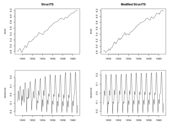
My view is that the non-diagonal matrix may have a point when the optimization algorithm does not converge for the standard design of the matrix. However, once the parameters have been estimated, the components should be extracted running the Kalman filter or smoother with a diagonal matrix. Otherwise, the estimate at the beginning of the sample will look quite erratic. See the Figure below. The left-hand-side plot is the output from StructTS while right-hand-side plot displays the estimated components for the same variation except that a the off-diagonal elements in the initial covariance matrix are set to zero.

Conclusion The point that I wanted to show in this point is that the choice of particular issues in the process of fitting the model may have an effect on the results. Most of these issues are often overlooked in the description of applications, making it difficult to reproduce the results obtained by others. The design of the procedure concerns not only the reproducibility of results, it may also affect the quality of results.